Week 2 Central Limit

Central Limit Theorem Exercises

For these exercises, we will be using the following dataset:

library(downloader) 
url <- "https://raw.githubusercontent.com/genomicsclass/dagdata/master/inst/extdata/mice_pheno.csv"
filename <- basename(url)
download(url, destfile=filename)
dat <- na.omit( read.csv(filename) ) 

Central Limit Theorem Exercises #1

1 point possible (graded)

If a list of numbers has a distribution that is well approximated by the normal distribution, what proportion of these numbers are within one standard deviation away from the list's average?

Answer: 0.682

pnorm(1)-pnorm(-1)

 

Central Limit Theorem Exercises #2

1/1 point (graded)

What proportion of these numbers are within two standard deviations away from the list's average?

Answer: 0.945

pnorm(2)-pnorm(-2)
 
 

Central Limit Theorem Exercises #3

1 point possible (graded)

What proportion of these numbers are within three standard deviations away from the list's average?

 Answer: 0.99

pnorm(3) - pnorm(-3)

Central Limit Theorem Exercises #4

1 point possible (graded)

Define y to be the weights of males on the control diet. What proportion of the mice are within one standard deviation away from the average weight (remember to use popsd for the population sd)?

 Answer: 0.6950673

y <- filter(dat, Sex=="M" & Diet=="chow") %>% select(Bodyweight) %>% unlist
z <- ( y - mean(y) ) / popsd(y)
mean( abs(z) <=1 )

Central Limit Theorem Exercises #5

1 point possible (graded)

What proportion of these numbers are within two standard deviations away from the list's average?

Answer:   0.9461883

mean( abs(z) <=2)

Central Limit Theorem Exercises #6

1 point possible (graded)

What proportion of these numbers are within three standard deviations away from the list's average?

Answer: 0.9910314

mean( abs(z) <=3 )

Central Limit Theorem Exercises #7

1/1 point (graded)

Note that the numbers for the normal distribution and our weights are relatively close. Also, notice that we are indirectly comparing quantiles of the normal distribution to quantiles of the mouse weight distribution. We can actually compare all quantiles using a qqplot. Which of the following best describes the qq-plot comparing mouse weights to the normal distribution?

qqnorm(z)
abline(0,1)

The points on the qq-plot fall exactly on the identity line.

The average of the mouse weights is not 0 and thus it can't follow a normal distribution.

The mouse weights are well approximated by the normal distribution, although the larger values (right tail) are larger than predicted by the normal. This is consistent with the differences seen between question 3 and 6. correct

These are not random variables and thus they can't follow a normal distribution.

Central Limit Theorem Exercises #8

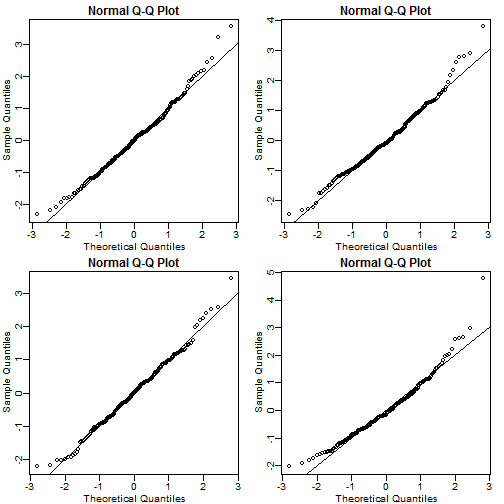
1/1 point (graded)

Create the above qq-plot for the four populations: male/females on each of the two diets. What is the most likely explanation for the mouse weights being well approximated? What is the best explanation for all these being well approximated by the normal distribution?

mypar(2,2)
y <- filter(dat, Sex=="M" & Diet=="chow") %>% select(Bodyweight) %>% unlist
z <- ( y - mean(y) ) / popsd(y)
qqnorm(z);abline(0,1)
y <- filter(dat, Sex=="F" & Diet=="chow") %>% select(Bodyweight) %>% unlist
z <- ( y - mean(y) ) / popsd(y)
qqnorm(z);abline(0,1)
y <- filter(dat, Sex=="M" & Diet=="hf") %>% select(Bodyweight) %>% unlist
z <- ( y - mean(y) ) / popsd(y)
qqnorm(z);abline(0,1)
y <- filter(dat, Sex=="F" & Diet=="hf") %>% select(Bodyweight) %>% unlist
z <- ( y - mean(y) ) / popsd(y)
qqnorm(z);abline(0,1)

The CLT tells us that sample averages are approximately normal.

This just happens to be how nature behaves in this particular case. Perhaps the result of many biological factors averaging out. correct

Everything measured in nature follows a normal distribution.

Measurement error is normally distributed.

Central Limit Theorem Exercises #9

1/1 point (graded)

Here we are going to use the function replicate to learn about the distribution of random variables. All the above exercises relate to the normal distribution as an approximation of the distribution of a fixed list of numbers or a population. We have not yet discussed probability in these exercises. If the distribution of a list of numbers is approximately normal, then if we pick a number at random from this distribution, it will follow a normal distribution. However, it is important to remember that stating that some quantity has a distribution does not necessarily imply this quantity is random. Also, keep in mind that this is not related to the central limit theorem. The central limit applies to averages of random variables. Let's explore this concept.

We will now take a sample of size 25 from the population of males on the chow diet. The average of this sample is our random variable. We will use the replicate to observe 10,000 realizations of this random variable. Set the seed at 1, generate these 10,000 averages. Make a histogram and qq-plot of these 10,000 numbers against the normal distribution.

We can see that, as predicted by the CLT, the distribution of the random variable is very well approximated by the normal distribution.

    y <- filter(dat, Sex=="M" & Diet=="chow") %>% select(Bodyweight) %>% unlist
    avgs <- replicate(10000, mean( sample(y, 25)))
    mypar(1,2)
    hist(avgs)
    qqnorm(avgs)
    qqline(avgs)

What is the average of the distribution of the sample average?

 Answer: 30.95581

 

mean(avgs)

Central Limit Theorem Exercises #10

1/1 point (graded)

What is the standard deviation of the distribution of sample averages?

Answer:  0.8368192

popsd(avgs)

CLT and t-distribution in Practice Exercises

Exercises 3-13 use the mouse data set we have previously downloaded:

library(downloader)
url <- "https://raw.githubusercontent.com/genomicsclass/dagdata/master/inst/extdata/femaleMiceWeights.csv"
filename <- "femaleMiceWeights.csv"
if(!file.exists("femaleMiceWeights.csv")) download(url,destfile=filename)
dat <- read.csv(filename)

CLT and t-distribution in Practice Exercises #1

1 point possible (graded)

The CLT is a result from probability theory. Much of probability theory was originally inspired by gambling. This theory is still used in practice by casinos. For example, they can estimate how many people need to play slots for there to be a 99.9999% probability of earning enough money to cover expenses. Let's try a simple example related to gambling.
Suppose we are interested in the proportion of times we see a 6 when rolling n=100 die. This is a random variable which we can simulate with x=sample(1:6, n, replace=TRUE) and the proportion we are interested in can be expressed as an average: mean(x==6). Because the die rolls are independent, the CLT applies.
We want to roll n dice 10,000 times and keep these proportions. This random variable (proportion of 6s) has mean p=1/6 and variance p*(1-p)/n. So according to CLT z = (mean(x==6) - p) / sqrt(p*(1-p)/n) should be normal with mean 0 and SD 1. Set the seed to 1, then use replicate to perform the simulation, and report what proportion of times z was larger than 2 in absolute value (CLT says it should be about 0.05).

Answer: 0.0424

set.seed(1)
n <- 100
sides <- 6
p <- 1/sides
zs <- replicate(10000,{
  x <- sample(1:sides,n,replace=TRUE)
  (mean(x==6) - p) / sqrt(p*(1-p)/n)
}) 
qqnorm(zs)
abline(0,1)#confirm it's well approximated with normal distribution
mean(abs(zs) > 2)

CLT and t-distribution in Practice Exercises #2

1/1 point (graded)

For the last simulation you can make a qqplot to confirm the normal approximation. Now, the CLT is an asympototic result, meaning it is closer and closer to being a perfect approximation as the sample size increases. In practice, however, we need to decide if it is appropriate for actual sample sizes. Is 10 enough? 15? 30?

In the example used in exercise 1, the original data is binary (either 6 or not). In this case, the success probability also affects the appropriateness of the CLT. With very low probabilities, we need larger sample sizes for the CLT to "kick in".

Run the simulation from exercise 1, but for different values of p and n. For which of the following is the normal approximation best?

p=0.5 and n=5

p=0.5 and n=30 correct

p=0.01 and n=30

p=0.01 and n=100

ps <- c(0.5,0.5,0.01,0.01)
ns <- c(5,30,30,100)
library(rafalib)
mypar(4,2)
for(i in 1:4){
  p <- ps[i]
  sides <- 1/p
  n <- ns[i]
  zs <- replicate(10000,{
  	x <- sample(1:sides,n,replace=TRUE)
  	(mean(x==1) - p) / sqrt(p*(1-p)/n)
  }) 
  hist(zs,nclass=7)
  qqnorm(zs)
  abline(0,1)
}

CLT and t-distribution in Practice Exercises #3

1/1 point (graded)

As we have already seen, the CLT also applies to averages of quantitative data. A major difference with binary data, for which we know the variance is $p(1-p)$, is that with quantitative data we need to estimate the population standard deviation.

In several previous exercises we have illustrated statistical concepts with the unrealistic situation of having access to the entire population. In practice, we do *not* have access to entire populations. Instead, we obtain one random sample and need to reach conclusions analyzing that data. dat is an example of a typical simple dataset representing just one sample. We have 12 measurements for each of two populations:

    X <- filter(dat, Diet=="chow") %>% select(Bodyweight) %>% unlist
    Y <- filter(dat, Diet=="hf") %>% select(Bodyweight) %>% unlist

We think of $X$ as a random sample from the population of all mice in the control diet and $Y$ as a random sample from the population of all mice in the high fat diet.

Define the parameter ${\mu }_X$ as the average of the control population. We estimate this parameter with the sample average $\overline{X}$. What is the sample average?

 Answer:  23.8113

mean(X)

CLT and t-distribution in Practice Exercises #4

1/1 point (graded)

We don't know ${\mu }_X$ , but want to use $\overline{X}$ to understand ${\mu }_X$. Which of the following uses CLT to understand how well $\overline{X}$ approximates ${\mu }_X$ ?

$\overline{X}$ follows a normal distribution with mean 0 and standard deviation 1.

${\mu }_X$ follows a normal distribution with mean $\overline{X}$ and standard deviation $\frac{{\sigma }_X}{\sqrt{12}}$ where ${\sigma }_X$ is the population standard deviation.

$\overline{X}$ follows a normal distribution with mean ${\mu }_X$ and standard deviation ${\sigma }_X$ where ${\sigma }_X$ is the population standard deviation.

$\overline{X}$ follows a normal distribution with mean ${\mu }_X$ and standard deviation $\frac{{\sigma }_X}{\sqrt{12}}$ where ${\sigma }_X$ is the population standard deviation. correct

CLT and t-distribution in Practice Exercises #5

1/1 point (graded)

The result above tells us the distribution of the following random variable: What does the CLT tell us is the mean of Z$$ (you don't need code)?

Answer: 0 

CLT and t-distribution in Practice Exercises #6

1 point possible (graded)

The result of 4 and 5 tell us that we know the distribution of the difference between our estimate and what we want to estimate, but don't know. However, the equation involves the population standard deviation

, which we don't know. Given what we discussed, what is your estimate of ?

 Answer: 3.022541

 
sd(X)
 

 Answer:  0.02189533

2 * ( 1-pnorm(2/sd(X) * sqrt(12) ) )
 

 Answer:  1.469867

sqrt( sd(X)^2/12 + sd(Y)^2/12 )
##or sqrt( var(X)/12 + var(Y)/12)
 
 

 Answer:  2.055174

 
( mean(Y) - mean(X) ) / sqrt( var(X)/12 + var(Y)/12)
##or t.test(Y,X)$stat
 
 

For some of the following exercises you need to review the t-distribution that was discussed in the lecture. If you have not done so already,  you should review the related book chapters from our textbook which can also be found here and here.
In particular, you will need to remember that the t-distribution is centered at 0 and has one parameter: the degrees of freedom, that control the size of the tails. You will notice that if X follows a t-distribution the probability that X is smaller than an extreme value such as 3 SDs away from the mean grows with the degrees of freedom. For example, notice the difference between:

1 - pt(3,df=3)
1 - pt(3,df=15)
1 - pt(3,df=30)
1 - pnorm(3)

As we explained, under certain assumptions, the t-statistic follows a t-distribution. Determining the degrees of freedom can sometimes be cumbersome, but the t.test function calculates it for you. One important fact to keep in mind is that the degrees of freedom are directly related to the sample size. There are various resources for learning more about degrees of freedom on the internet as well as statistics books.

CLT and t-distribution in Practice Exercises #10

1/1 point (graded)

If we apply the CLT, what is the distribution of this t-statistic?

Normal with mean 0 and standard deviation 1. correct

t-distributed with 22 degrees of freedom.

Normal with mean 0 and standard deviation

.

t-distributed with 12 degrees of freedom.

CLT and t-distribution in Practice Exercises #11

1/1 point (graded)

Now we are ready to compute a p-value using the CLT. What is the probability of observing a quantity as large as what we computed in 9, when the null distribution is true?

Answer: 0.0398622

Z <- ( mean(Y) - mean(X) ) / sqrt( var(X)/12 + var(Y)/12)
2*( 1-pnorm(Z)) 

CLT and t-distribution in Practice Exercises #12

1/1 point (graded)

CLT provides an approximation for cases in which the sample size is large. In practice, we can't check the assumption because we only get to see 1 outcome (which you computed above). As a result, if this approximation is off, so is our p-value. As described earlier, there is another approach that does not require a large sample size, but rather that the distribution of the population is approximately normal. We don't get to see this distribution so it is again an assumption, although we can look at the distribution of the sample with qqnorm(X) and qqnorm(Y). If we are willing to assume this, then it follows that the t-statistic follows t-distribution. What is the p-value under the t-distribution approximation? Hint: use the t.test function.

Answer: 0.053

t.test(X,Y)$p.value

CLT and t-distribution in Practice Exercises #13

1/1 point (graded)

With the CLT distribution, we obtained a p-value smaller than 0.05 and with the t-distribution, one that is larger. They can't both be right. What best describes the difference?

A sample size of 12 is not large enough, so we have to use the t-distribution approximation.

These are two different assumptions. The t-distribution accounts for the variability introduced by the estimation of the standard error and thus, under the null, large values are more probable under the null distribution. correct

The population data is probably not normally distributed so the t-distribution approximation is wrong.

Neither assumption is useful. Both are wrong.